Random Search vs. Bayesian Optimization

In this section, we demonstrate the behaviors of random search and Bayesian optimization in a simple simulation environment.

Create a Reward Function for Toy Experiments

• Import the packages:

import numpy as np
import matplotlib.pyplot as plt
from mpl_toolkits.mplot3d import Axes3D

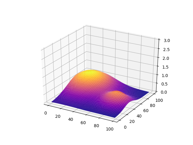
• Generate the simulated reward as a mixture of 2 gaussians:

Input Space x = [0: 99], y = [0: 99]. The rewards is a combination of 2 gaussians as shown in the following figure:

def gaussian2d(x, y, x0, y0, xalpha, yalpha, A):
    return A * np.exp( -((x-x0)/xalpha)**2 -((y-y0)/yalpha)**2)

x, y = np.linspace(0, 99, 100), np.linspace(0, 99, 100)
X, Y = np.meshgrid(x, y)

Z = np.zeros(X.shape)
ps = [(20, 70, 35, 40, 1),
      (80, 40, 20, 20, 0.7)]
for p in ps:
    Z += gaussian2d(X, Y, *p)

• Visualize the reward space:

fig = plt.figure()
ax = fig.gca(projection='3d')
ax.plot_surface(X, Y, Z, cmap='plasma')
ax.set_zlim(0,np.max(Z)+2)
plt.show()

Create Training Function

We can simply define an AutoTorch searchable function with a decorator at.gargs. The reporter is used to communicate with AutoTorch search and scheduling algorithms.

import autotorch as at

@at.args(
    x=at.Int(0, 99),
    y=at.Int(0, 99),
)
def toy_simulation(args, reporter):
    x, y = args.x, args.y
    reporter(accuracy=Z[y][x])

Random Search

random_scheduler = at.scheduler.FIFOScheduler(toy_simulation,
                                              resource={'num_cpus': 1, 'num_gpus': 0},
                                              num_trials=30,
                                              reward_attr="accuracy",
                                              resume=False)
random_scheduler.run()
random_scheduler.join_jobs()
print('Best config: {}, best reward: {}'.format(random_scheduler.get_best_config(), random_scheduler.get_best_reward()))

Out:

Best config: {'x': 22, 'y': 72}, best reward: 0.9942633286025881

Bayesian Optimization

bayesopt_scheduler = at.scheduler.FIFOScheduler(toy_simulation,
                                                searcher='bayesopt',
                                                resource={'num_cpus': 1, 'num_gpus': 0},
                                                num_trials=30,
                                                reward_attr="accuracy",
                                                resume=False)
bayesopt_scheduler.run()
bayesopt_scheduler.join_jobs()
print('Best config: {}, best reward: {}'.format(bayesopt_scheduler.get_best_config(), bayesopt_scheduler.get_best_reward()))

Out:

Best config: {'x': 20, 'y': 70}, best reward: 1.000009105108358

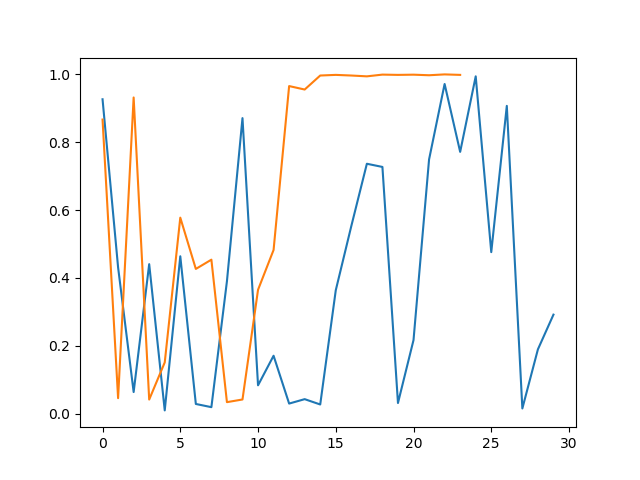
Compare the performance

Get the result history:

results_bayes = [v[0]['accuracy'] for v in bayesopt_scheduler.training_history.values()]
results_random = [v[0]['accuracy'] for v in random_scheduler.training_history.values()]

fig = plt.figure()
plt.plot(range(len(results_random)), results_random, range(len(results_bayes)), results_bayes)
plt.show()

Advance Usage for Bayesian Optimization

For some special cases, not all configurations are valid for the requirement. Instead of falling back to random search, we can pre-generate a set of valid configurations using random search, and accelerate the HPO using Bayesian Optimization. The key idea is fitting GP model using observed data points, and using acqusition function to re-rank the pending configurations.

• Define valid condiction

We require x or y to be an even number

def is_valid_config(config):
    return config['x'] % 2 == 0 or config['y'] % 2 == 0

• Pre-generate configurations using random searcher

random_searcher = at.searcher.RandomSearcher(toy_simulation.cs)

lazy_configs = []
valid_cnt = 0

while valid_cnt < 500:
    config = random_searcher.get_config()
    if is_valid_config(config):
        valid_cnt += 1
        lazy_configs.append(config)

• Initialize lazy configurations with Bayesian optimization

lazy_bayes = at.searcher.BayesOptSearcher(toy_simulation.cs, lazy_configs=lazy_configs)

lazy_scheduler = at.scheduler.FIFOScheduler(toy_simulation,
                                            searcher=lazy_bayes,
                                            resource={'num_cpus': 1, 'num_gpus': 0},
                                            num_trials=20,
                                            reward_attr="accuracy",
                                            resume=False)
lazy_scheduler.run()
lazy_scheduler.join_jobs()
print('Best config: {}, best reward: {}'.format(lazy_scheduler.get_best_config(), lazy_scheduler.get_best_reward()))

Out:

Best config: {'x': 20, 'y': 73}, best reward: 0.9943964671954428

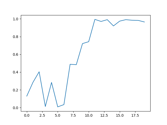
• Plot the training curve

fig = plt.figure()
results_lazy = [v[0]['accuracy'] for v in lazy_scheduler.training_history.values()]
plt.plot(range(len(results_lazy)), results_lazy)
plt.show()